Introduction
Functional Coverage in SystemVerilog
In SystemVerilog a fundamental coverage unit is a coverpoint. It contains several bins and each bin may contain several values. Every coverpoint is associated with a variable or signal. At sampling event, the coverpoint variable value is compared with each defined bin. If there is a match, then the number of hits of the particular bin is incremented. Coverpoints are organized in covergroups, which are specific class-like structures. A single covergroup may have several instances and each instance may collect coverage independently. A covergroup requires sampling, which may be defined as a logic event (e.g. a positive clock edge). Sampling may also be called implicitly in the testbench procedural code by invoking a sample() method of the covergroup instance. A bin may be also defined as an ignore_bins, which means its match does not increase a coverage count, or an illegal_bins, which results in error when hit during the test execution.
Another coverage construct in SystemVerilog is a cross. It automatically generates a Cartesian product of bins from several coverpoints. It is a useful feature simplifying the functional coverage generation. As it may be difficult or unnecessary to cover all the cross-bins, some of them may be excluded from the analysis. This is possible using the binsof … intersect syntax.
The most important limitations of the SystemVerilog functional coverage features are:
straightforward bins matching criteria – only satisfied by equality or inclusion relation;
bins may be only constants or transitions (possibly wildcard);
flat coverage structure – cover groups cannot contain other cover groups, which would correspond better to a verification plan scheme;
not possible to get the detailed coverage information in real time (e.g. when a specific bin was hit).
Functional Coverage with cocotb-coverage
The general assumptions for the architecture of the functional coverage features are as follows:
functional coverage structure should better match a real verification plan;
its syntax should be more flexible, but a separation between coverage and executable code should be maintained;
features for analysing the coverage during test execution should be added or extended;
coverage primitives should be able to monitor testbench objects at a higher level of abstraction.
The implemented mechanism is based on the idea of decorator design pattern.
In Python, a decorator syntax is readable and easy to use.
Instead of sampling coverage items by an additional method, decorators are
by default invoked at each decorated function call.
As it is easy to create functions in Python
(for example anonymous functions can be created as lambda expressions –
single-line function definitions), this is a convenient solution.
The coverage structure is based on a prefix tree (a trie).
The main coverage primitive is a CoverItem, which corresponds to a SystemVerilog covergroup.
CoverItem may contain other CoverItems or objects extending CoverItems base class,
which are CoverPoints, CoverCrosses or arbitrary new, user-defined types.
CoverItems are created automatically,
the user defines only CoverPoint or CoverCross primitives (the lowest level nodes in the trie).
Each created primitive has a unique ID – a dot-separated string.
This string denotes the position of an object in the coverage trie.
For example, a CoverPoint a.b.c is a member of the a.b CoverItem,
which is then a member of the a CoverItem.
The structure of the coverage trie is presented below.
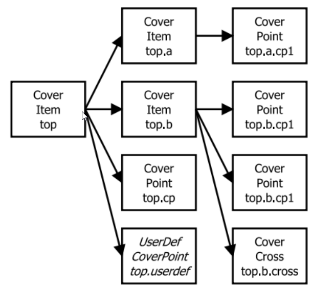
An example of the coverage trie structure
A CoverPoint decorator functionality corresponds to a coverpoint in SystemVerilog.
It checks whether the arguments of a decorated function match the predefined bins.
In a simple case, variables equality to the bins is checked.
Additionally, it is possible to define:
a transformation function, which transforms the arguments of a decorated function and the transformation result is compared to the bins,
a relation function, which defines the binary relation of bin comparison (which by default is the equality operator).
Bins in the CoverPoint may be a list of arbitrary objects which are hashable.
In Python they are constants, tuples or even functions.
In general, the bins matching condition can be described by a formula:
relation(transformation(arguments), bin) is True
A CoverCross decorator functionality corresponds to a cross in SystemVerilog.
Its main attributes are a list of items (CoverPoints),
a list of bins to be ignored and an optional ignore relation function.
CoverCross bins are tuples generated as a Cartesian product of bins from CoverPoint items.
An item in (ign_bins) may contain a None object which corresponds to
binsof … intersect syntax, meaning a specific CoverPoint bin value may be a wildcard.
An example below presents the same coverage implementation in SystemVerilog and in Python.
As the CoverPoint length bins contain value range,
a relation must be defined in the Python implementation, which uses a tuple (in this case a pair)
and finds out whether the variable is within a given range.
Original SystemVerilog code
covergroup transfer;
  direction : coverpoint dir {
      bins read  = {0};
      bins write = {1};
  }
  length : coverpoint length {
      bins short = {[1:10]};
      bins long  = {[10:100]};
  }
  type : coverpoint type {
      bins type_a = {A};
      bins type_b = {B};
  }
  tr_cross : cross
      direction, length, type {
      ignore_bins ign = binsof(type) intersect {A};
  }
|
Equivalent Python code
@CoverPoint ("transfer.direction" ,
    xf = lambda xfer: xfer.dir,
    bins = [0, 1]
)
@CoverPoint ("transfer.length",
    xf = lambda xfer: xfer.length,
    bins = [(1, 10), (10, 100)],
    rel = lambda val, b: b(0) <= val <= b(1)
)
@CoverPoint("transfer.type",
    xf = lambda xfer: xfer.type,
    bins = [A, B]
)
@CoverCross("transfer.tr_cross",
    items = ["transfer.direction",
             "transfer.length",
             "transfer.type"],
    ign_bins = [(None, None, A)]
)
def decorated_function(xfer):
    ...
|
More complex examples of coverage mechanisms are presented below.
The coverage.transition defines a transformation by a transition_inta() function.
This function returns a tuple containing the previous and the current value of inta.
It is a simple example of the transition bins.
The coverage.primefactors defines a relation by a function has_prime_factor()
checking if a bin value is a prime factor of inta.
The inj attribute is set True, which means that more than one bin can be matched at a single sampling.
For example, an inta value of 30 matches bins 2, 3, and 5.
The coverage.tuple presents how arbitrary hashable type may be used as a bins.
The bins are predefined in a simple bins list containing 40 elements of (int, string) pairs.
The coverage.check is an example of a higher-level assertion.
This is a new defined coverage primitive which checks whether the string variable is not empty.
If at least one empty string is sampled, coverage level is forced zero.
simple_bins = []  # bins generation for coverage.tuple: create a 40-elements list
for i in range(1, 21):  # for i=1 to 20
    simple_bins.extend([(i, 'y'), (i, 'n')])  # extend list by two elements - tuples(int, str)

# transition function for coverage.transition
prev_value=0  # previous value defined outside the function (global variable)
def transition_inta(inta, intb, string):  # function definition
    transition = (prev_value, inta)  # transition as a tuple of(int, int)
    prev_value = inta  # update previous value
    return transition

# sampling function and its coverage decorators
@CoverPoint("coverage.transition", xf=transition_inta, bins=[(1, 2), (2, 3), (3, 4)])
@CoverPoint("coverage.primefactors",xf=lambda inta, intb, string: inta,
    rel=has_prime_factor, inj=True, bins=[2, 3, 5, 7, 11, 13, 17])
@CoverPoint("coverage.tuple", xf=lambda inta, intb, string: (inta+intb, string),
    bins=simple_bins)
@CoverCheck("coverage.check",f_fail=lambda inta, intb, string: string == "")
def decorated_function(inta, intb, string):
    ...
There are some higher-level functions available for CoverItems.
They can be used in real time in the testbench, which allows for processing coverage data dynamically.
It is possible to easily get the coverage data from each primitive or define a callback,
called when coverage level has been exceeded or a specific bin was hit.
Callbacks may be used in order to adjust a test scenario when specific coverage goal has been achieved.
Instead of monitoring the coverage during the test execution,
a callback function will be called automatically.
A callback function may be simply appended to any CoverItem primitive by the testbench designer.
There are two types of callbacks:
threshold callback - called when
CoverItemexceeded given percentage threshold (seeadd_threshold_callback);bins callback - called when a specific bin in
CoverItemis hit (seeadd_bins_callback);
Note
More information about functional coverage background and this implementation can be found in
M. Cieplucha and W. Pleskacz, “New architecture of the object-oriented functional coverage mechanism for digital verification,” in 2016 1st IEEE International Verification and Security Workshop (IVSW), July 2016, pp. 1–6.
Constrained Random Verification Features in SystemVerilog
SystemVerilog users may define random variables using the rand/randc modifier. Calling randomize() function on a class instance (object) results in picking random values of the defined random variables, satisfying given constraints. Also a with modifier can be used together with randomize() which allow for appending additional constraints dynamically. Constraints are defined in a special section in the class named constraint. They describe a range values that a single variable may have or a relation between variables. It is also possible to define solution ranges with weights (using dist modifier). The solve … before is an additional construction which organizes variable randomization order.
Constraints are unique constructs of SystemVerilog. They are class members, but they are not functions or objects. Basic operations can be performed on constraints, such as enable/disable or inheritance. Soft constraints have been introduced in SystemVerilog 2012. They are resolved only when it is possible to satisfy them together with all other hard constrains. Every SystemVerilog simulator must implement a constraint solver. Although many open-source constraint solvers are available, testbench designers cannot use them, as they have no control over the simulator engine. The most important limitations of the existing constrained randomization features are related to their fixed syntax.
In cocotb-coverage, it is assumed that a constraint may be any callable object –
an arbitrary function or a class with __call__ method.
It allows for creating various functionalities quite easily and manipulating them in a flexible way.
Constrained Random Verification Features in cocotb-coverage
The main assumption for the constrained randomization features was to provide only a flexible API, and let the testbench designer to adjust it depending on project needs. There is an open-source based hard constraint solver used by this framework: python-constraint.
The general idea of cocotb-coverage is that all classes that intended
to use randomized variables should extend the base class Randomized.
Afterwards, random variables and their ranges should be defined.
Constraints are just arbitrary functions with only one requirement:
their argument names must match class member names.
It is possible to define two types of constraints:
functions that return a
True/Falsevalue, corresponding to SystemVerilog hard constraints;functions that return a numeric value, corresponding to a variables distribution (or cross-distribution) which also may be used as soft constraints.
The Randomized class API consists of the following functions:
add_rand(var, domain)- specifies var as a randomized variable taking values from the domain list;add_constraint(cstr)- adds a constraint function to the solver;del_constraint(cstr)- removes a constraint function from the solver;solve_order(vars0, vars1 ...)- optionally specifies the order of randomizing variables (can be used for problem decomposition or in case some random variables must be fixed before randomizing the others);pre_randomize- function called beforerandomize/randomize_with, corresponding to similar function in SV;post_randomize- function called afterrandomize/randomize_with, corresponding to similar function in SV;randomize()- main function that picks random values of the variables satisfying added constraints;randomize_with(cstr0, cstr1 ...)- similar torandomize(), but satisfies additional given constraints.
The example below presents the corresponding implementation of the randomized class with use of hard constraints.
Original SystemVerilog code
class rand_frame;
    typedef enum {SMALL, MED, BIG } size_t;
    rand logic [15:0] length;
    rand logic [15:0] pld;
    rand size_t size;
    constraint frame_sizes {
    if (size==MED) {
        length >= 64;
        length < 2000;
    } else if (size==SMALL) {
        length > 0;
        length < 64;
    } else if (size==BIG) {
        length >= 2000;
        length < 5000;
    }
        pld < length;
        pld % 2 == 0;
    }
endclass
|
Equivalent Python code
class rand_frame(crv.Randomized):
    def __init__(self):
        crv.Randomized.__init__(self)
        self.length = 0
        self.pld = 0
        self.size = "SMALL"
        self.add_rand("size", ["SMALL", "MED", "BIG"])
        self.add_rand("length", list(range(1, 5000)))
        self.add_rand("pld", list(range(0, 4999)))
        def frame_sizes(length, size):
            if (size=="SMALL") return length < 64
            elif (size=="MED") return 64 <= length < 2000
            else return length >= 2000
        self.add_constraint(frame_sizes)
        self.add_constraint(
            lambda length, pld: pld < length
        )
        self.add_constraint(lambda pld: pld % 2 == 0)
|
A more complex example is presented below. The class TripleInt contains three unsigned integer members,
y and z are randomized.
The first defined constraint combines all variables (random and non-random).
The second constraint defines a triangular distribution for variable z.
It is achieved by defining a function that has its maximum in the middle of the variable range (for solution z = 500).
The third one is a cross-distribution of variables y and z.
The weight function defines higher probability for solutions with higher difference between both variables.
The last one is a kind of a soft constraint –
very low probability is set for condition x > y,
which means that solutions satisfying x ≤ y will be strongly preferred.
class TripleInt(crv.Randomized):
    def __init__(self, x):
        crv.Randomized.__init__(self)
        self.x = x  # this is a non-random value, determined at class instance creation
        self.y = 0
        self.z = 0
        add_rand(y, list(range(1000)))  # 0 to 999
        add_rand(z, list(range(1000)))  # 0 to 999
        add_constraint(lambda x, y, z: x+y+z==1000)          # hard constraint
        add_constraint(lambda z: 500 - abs(500-z))           # triangular distribution of z variable
        add_constraint(lambda y, z: 100 + abs(y-z))          # multi-dimensional distribution
        add_constraint(lambda x, y: 0.01 if (y > x) else 1)  # soft constraint
It is assumed that only one hard constraint and one distribution may be associated with
each set of random variables.
So, for the example presented above, it is possible to define no more than six constraint functions:
separately for variables y and z and both (y and z).
It means that constraints may be overwritten, for example by randomize_with() function arguments.